Differences between Local Spatial Statistics Results

[PhilipGibbons]

Hi All,

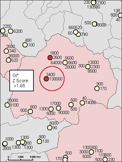
I have been doing some analysis of monitoring points to find clusters of high concentrations of pollutant values.  I have been exploring the results of the local spatial statistics tools (Local Moran's I and Gi*).  The results seem to contradict each other in places.  For example, mapping out the results of the local Moran's I values shows that a monitoring point has a negative Moran's I value, which means that it is surrounded by dissimilar values (Figure 1-the numbers next to the points are the raw monitoring values and the point circled in red is the point in question).  I also mapped out the Z Scores of the local Moran's I analysis to see which values were statistically significant (Figure 2).  Lastly, when running the hot spot analysis (Gi*) on my data set, the point in question received a high positive Z Score which means it is a statistically significant cluster of high values (Figure 3).  These results seem contradictory to me.  Why would the point be a part of a statistically significant cluster of high values when it is surrounded by dissimilar values?

Thanks for any and all help!

-Phil

[Anonymous User]

Original User: lrosenshein

Hi Phil,

This is a great question!  First of, it is important to understand that these two methods, Local Moran's I and Getis-Ord Gi*, while they are similar in terms of the types of questions that they answer, have some key differences that can explain why you would get such different results.  The main difference is that for Local Moran's I, when doing the analysis for each individual feature, the value of the feature being analyzed is NOT included in that analysis...only the neighboring values are.  Alternatively, when the local analysis is being done with Getis-Ord Gi*, the value of each feature is included in its own analysis.  In other words, the local mean for Moran's I includes only neighboring features, whereas the local mean for Getis-Ord Gi* includes all features, including the one in question. 

So, when doing a hot spot analysis using Getis-Ord Gi*, if you have chosen a scale for your analysis that is small, even though there are features around with low values, it is definitely conceivable that a feature with a very high value would show up as a hot spot even though it is surrounded by low values (essentially the value of the feature is so high that it brings the local mean up).  Alternatively, it makes sense that the same feature, when analyzed using Local Moran's I, would show up as a High surrounded by Low values.  Essentially, both analyzes are right, it just depends on the question that you're asking which result makes sense for you.

It is very important to think about the scale of the questions that you're asking and make sure that the distance that you're choosing (or the number of neighbors if you're using k-nearest neighbors) is appropriate for the question that you're asking and the spatial patterns you're looking for.  The size of the neighborhoods will greatly influence the results, and it is very important to think about that when choosing an appropriate distance band or neighbor count. 

You can take a look at the math behind the hot spot analysis tool here: How Hot Spot Analysis Works, and the Local Moran's I tool here: How Cluster and Outlier Analysis Works.  You can also find a tool for picking a scale for your analysis here: Supplementary Spatial Statistics Toolbox for ArcGIS 10, the tool is called Incremental Spatial Autocorrelation.

Hope this helps.

Lauren Rosenshein
Geoprocessing Product Engineer